[This document is still under construction! The text is written but the graphics and videos are currently being authored. Check back soon for the finished article!]

Introduction

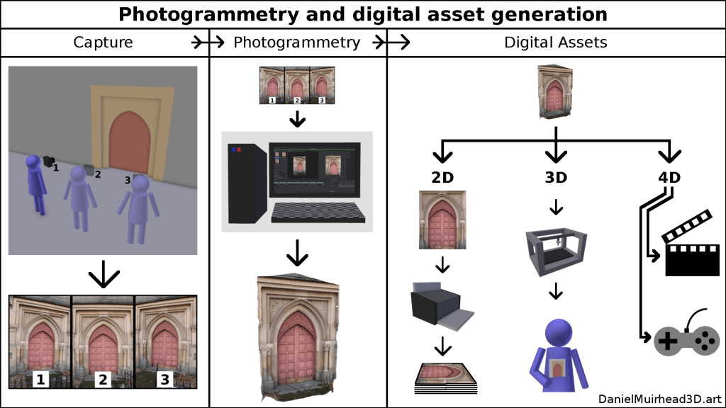
During this document, by ‘photogrammetry’ is meant using a computer program (photogrammetry software) to derive a virtual 3D model from a set of photographs of its real world equivalent.

A typical photogrammetry production process will involve:

1. photographing the real world subject from a variety of angles and positions;
2. using photogrammetry software to automatically reconstruct the subject as a virtual 3D model;
3. preparing the 3D model for a particular purpose or for use within a specific context, through further processing.

Equipment

• Digital camera (or camcorder);
• personal computer (capable of running the photogrammetry software);
• photogrammetry software (please see [forthcoming]).

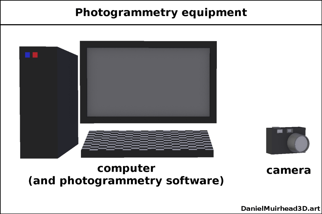
Photo capture

A photograph involves a camera capturing the interaction between a source of illumination and a surface. Light emits from a source, bounces off or into a subject, and the camera captures that interaction (from a specific position and orientation) in a photograph.

A successful photogrammetry reconstruction depends on good photos. The 3 variables implied above will influence how good a photograph is for use as a photogrammetry input:

• camera: the quality of the sensor and lens; image file encoding and data compression;
• illumination: bright, direct and focused (bad) or muted, diffuse and evenly spread (good);
• subject surface: shiny and reflective, self-identical, translucent (bad) or non-shiny and matte, uniquely-patterned, opaque (good).

[graphic: illumination; subject surface]

In addition to its surface, the subject’s geometry influences the performance of the capture. More specifically, if we consider a set of photographs as being captured from a succession of positions and orientations, and we define that succession as the ‘capture trajectory’, then the complexity of the capture trajectory co-varies with the complexity of the subject geometry. For example: if we have one subject that is shaped like a simple sphere or cube, then the capture trajectory will similarly be very simple; if we have a comparable subject of the same size but with many protrusions and recesses, then the capture trajectory would have to be adjusted to account for that more complex geometry.

[graphic: variance in capture trajectory as function of subject surface complexity]

Photogrammetry

Heads-up! This section is written from the perspective of a 3D artist and photogrammetry practitioner, not a computer vision scientist or software engineer. What is conveyed here is my understanding of the photogrammetry software process, informed by my practical experience of using several different softwares. This account of ‘the main photogrammetry stages’ is how I quantify and compare the performance of different softwares – but it may contain some inadvertent inaccuracies. In other words: for a deep understanding of what photogrammetry software is actually doing and how it actually works (in theory; on paper) the reader is recommended to consult additional sources.

Photogrammetry software involves the automated processing of a photo set through several main stages:

1. SPARSE (Structure from Motion, SfM) – calculations culminating in establishing the relative position and orientation of each photo in the set (the input photos or images are usually referred to as ‘cameras’), resulting in a 3D visualisation that depicts both that camera layout and an initial low quality reconstruction of the subject as a sparse point cloud;
2. DENSE (Multi-View Stereo, MVS) – building on that initial reconstruction, a different set of calculations that generates a higher quality reconstruction of the subject as a dense point cloud;
3. MESH (MVS continued) – from the dense point cloud is derived a surface model, namely a mesh (for the difference between point cloud models and mesh models, see both https://en.wikipedia.org/wiki/Point_cloud and https://en.wikipedia.org/wiki/Polygon_mesh), optionally this mesh might be coloured, the colours of the mesh surface being interpolated from the colour value of each point comprising the mesh (points are also called vertices, shortened to verts, so such a model is called a vert-coloured mesh);
4. TEXTURE – the surface of the model is ‘painted’ with reference to what is visible through the cameras, or, the subject as viewed through the cameras is projected onto the faces that comprise the subject surface (resulting in a model with ‘higher resolution’ colours than the vert-coloured mesh of the previous stage).

[graphic: SPARSE>DENSE>MESH (incl. vert-coloured)>TEXTURE]

This whole process, from photo set to textured 3D model, is completely automated, although it is possible for the technician to intervene after each stage to perform quality assurance or optimisations. For example (bearing in mind that with the obvious exception of ‘manual definition’ and ‘manual selection’, each of these processes in theory could also be automated according to pre-defined values and thresholds):

• after SPARSE, manual definition of bounding box for which part of the subject is to be reconstructed (to reduce processing time for subsequent stages);
• after DENSE (also after MESH), deletion of unwanted parts of the subject (via manual selection tools, or automated selection via ‘confidence’ values or point colour or similar, then deletion);
• after MESH, selection+deletion of unwanted parts, also decimation+retopology (reducing the mesh size then ‘averaging out’ the distribution of points and faces);
• after any of the stages, judging the quality of the output and if different to expected, re-running the software but at different settings (e.g. increasing accuracy of SPARSE or resolution of DENSE).

Optionally, at the MESH stage, the technician may generate both high quality (original) and low quality (through decimation+retopology) meshes. Then, during TEXTURE, perform texturing on the low quality mesh (thereby assigning texture coordinates), and transfer some of the high quality details onto the low quality mesh through the use of a Normal map or Bump map (which use those same texture coordinates). These maps are a special type of hidden texture that work behind the scenes in collaboration with the illumination sources of a lit virtual 3D scene (i.e. they are not relevant to rendering performed in a ‘shadeless’ or ‘unlit’ virtual environment), to cast shadows in a way that implies the presence of the geometry found in the high quality mesh. But that information is being conveyed through some Computer Generated Imagery trickery. (See https://en.wikipedia.org/wiki/Normal_mapping). This issue more falls under Further Processing (the section below) but it is worth mentioning at this juncture because some photogrammetry softwares come with the integrated ability to generate Normal/Bump Maps.

[graphic: high quality mesh, then decimated, then retoplogised]

[graphic: in a lit virtual environment, comparision of HQ mesh vs LQ mesh vs LQ+Normal mesh]

Further Processing

[do separate discussion, hyperlink, discussion re ‘product catalogue’/derived digital assets]

Photogrammetry software options

[do separate discussion, hyperlink]

Appendix: recommended capture trajectories

[XOR do separate discussion and provide hyperlink to that within ‘capture’ section above]